Coupled Free-Flow and Porous Media Flow Models in DuMux
Environmental and Agricultural Issues
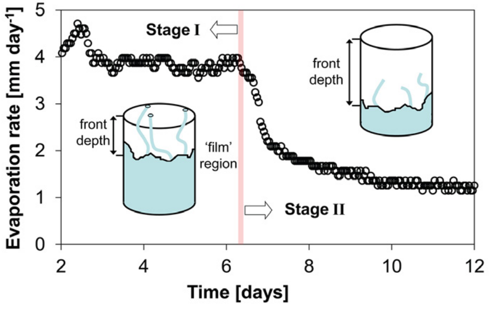
 Fig.1 - Evaporation of
soil water (Heck et al. (2020))1
Fig.1 - Evaporation of
soil water (Heck et al. (2020))1
- Evaporation of soil water
- Soil salinization
- Underground storage (e.g. CO2, atomic waste)
Technical Issues
 Fig.2 - Filter (Schneider et
al. (2023))2
Fig.2 - Filter (Schneider et
al. (2023))2
- Fuel cells
- Filters (e.g. air)
- Heat exchangers (e.g. CPU cooling)
Biological Issues
 Fig.3 - Brain tissue
(Koch et al. (2020))3
Fig.3 - Brain tissue
(Koch et al. (2020))3
- Brain tissue
- Leaf structure
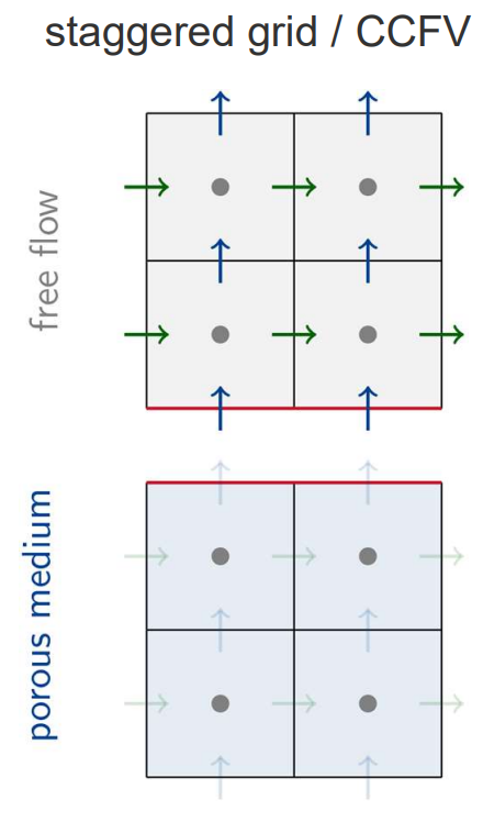
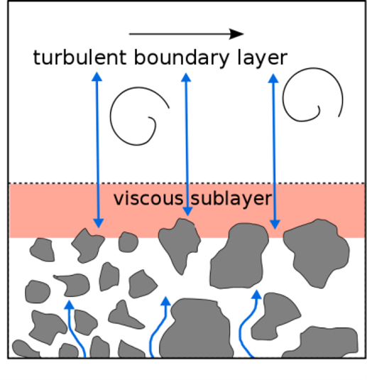
Conceptual Physical Model

Mathematical Model

Free Flow:
- Stokes / Navier-Stokes / RANS
- 1-phase, n-components, non-isothermal
Interface conditions:
- no thickness, no storage, local thermal equilibrium
- continuity of fluxes and state variables
Porous media:
- Darcy / Forchheimer
- m-phases, n-components, non-isothermal
Numerical Model
Eqs - Free Flow

Momentum balance (Navier-Stokes equation) \[ \frac{\partial \left(\rho_g \textbf{v}_g\right)}{\partial t} + \nabla \cdot (\rho_g \textbf{v}_g \textbf{v}_g^T) - \nabla \cdot \mathbf{\tau}_g +\nabla \cdot (p_g\textbf{I})- \rho_g \textbf{g} = 0 \]
Component mass balance \[ \frac{\partial \left(\rho_g X^\kappa_g\right)}{\partial t} + \nabla \cdot \left( \rho_g X^\kappa_g \textbf{v}_g + \mathbf{j}_{\text{diff}}^\kappa\right) - q^\kappa = 0 \]
Eqs - Free Flow
- Energy balance \[ \begin{aligned} \frac{\partial (\rho_g u_g) }{\partial t} + \nabla \cdot (\rho_g h_g \textbf{v}_g) &+ \sum_{\kappa} {\nabla \cdot (h_g^\kappa \textbf{j}_{\text{diff}}^\kappa)} \\ &- \nabla \cdot (\lambda_{g} \nabla T) = 0 \end{aligned} \]
Eqs - Porous Medium Flow

Darcy velocity (momentum balance) \[ \textbf{v}_\alpha = - \frac{k_{r,\alpha}}{\mu_\alpha} K \left(\nabla p_\alpha - \rho_\alpha \textbf{g}\right) \]
Component mass balance \[ \sum\limits_{\alpha \in \{\text{l, g} \}} \left(\phi \frac{\partial \left(\rho_\alpha S_\alpha X_\alpha^\kappa\right)}{\partial t } + \nabla \cdot \rho_\alpha X_\alpha^\kappa \textbf{v}_\alpha + \nabla \cdot \mathbf{j}_{\text{diff}}^\kappa\right) = 0 \]
Eqs - Porous Medium Flow
- Total energy balance \[ \begin{aligned} \sum\limits_{\alpha \in \{\text{l, g} \}} &\left(\phi\frac{\partial \left(\rho_\alpha S_\alpha u_\alpha\right)}{\partial t} + \nabla \cdot \left(\rho_\alpha h_\alpha \textbf{v}_\alpha \right)\right) \\ &+ \left(1-\phi\right) \frac{\partial \left(\rho_s c_{p,s}T\right)}{\partial t} - \nabla\cdot \left(\lambda_{pm} \nabla T \right) = 0 \end{aligned} \]
Eqs - Coupling Conditions

Continuity of total mass flux \[ [(\rho_g \textbf{v}_g) \cdot \textbf{n}]^{\text{ff}} = - [(\rho_g \textbf{v}_g + \rho_w \textbf{v}_w) \cdot \textbf{n}]^{\text{pm}} \]
Continuity of component flux \[ \begin{aligned} &\left[(\rho_g X_g^\kappa \textbf{v}_g + \textbf{j}_{\text{diff}^\kappa}) \cdot \textbf{n}\right]^{\text{ff}} = \\&- \left[\left( \sum_{\alpha} (\rho_{\alpha} X_{\alpha}^\kappa \textbf{v}_\alpha + \textbf{j}^\kappa_{\text{diff}, \alpha})\right) \cdot \textbf{n}\right]^{\text{pm}}\, \end{aligned} \]
Eqs - Coupling Conditions
Momentum condition in normal direction \[ \left[((\rho_g \textbf{v}_g \textbf{v}_g^T - \mathbf{\tau}_g + p_g\textbf{I}) \textbf{n} )\right]^{\text{ff}} = \left[(p_g\textbf{I})\textbf{n}\right]^{\text{pm}}\, \]
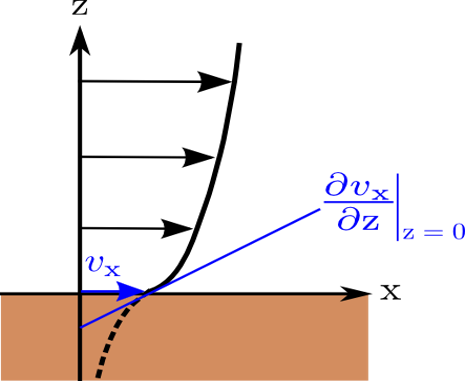
Momentum condition in tangential direction \[ \begin{aligned} \left[\left(- \textbf{v}_g - \frac{\sqrt{(\textbf{K}\textbf{t}_i)\cdot \textbf{t}_i}}{\alpha_{\mathrm{BJ}}} (\nabla \textbf{v}_g + \nabla \textbf{v}_g^T)\textbf{n} \right) \cdot \textbf{t}_i \right]^{\text{ff}} = 0\, , \\ \quad i \in \{1, .. ,\, d-1\}\, \end{aligned} \]
Eqs - Coupling Conditions
- Continuity of energy fluxes \[ \begin{aligned} \left[\left(\rho_g h_g \textbf{v}_g + \sum_i h_g^\kappa \textbf{j}_{\text{diff},g}^\kappa - \lambda_{g} \nabla T\right)\cdot \textbf{n}\right]^{\text{ff}} =\\ - \left[\left( \sum_\alpha (\rho_\alpha h_\alpha \textbf{v}_\alpha + \sum_\kappa h_\alpha^\kappa \textbf{j}_{\text{diff},\alpha}^\kappa) - \lambda_{\text{pm}}\nabla T\right)\cdot \textbf{n}\right]^{\text{pm}}\, \end{aligned} \]
Example: Soil-Water Evaporation
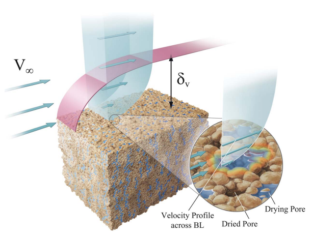
Example: Soil-Water Evaporation
Example: Simple Evaporation Setup

Tab1: Input parameter
| Parameter | Value |
|---|---|
| \(\textbf{v}_g^{ff}\) [m/s] | (3.5,0)\(^T\) |
| \(p_g^{ff}\) [Pa] | 1e5 |
| \(X_g^{w,ff}\) [-] | 0.008 |
| \(T^{ff}\) [K] | 298.15 |
| \(p_g^{pm}\) [Pa] | 1e5 |
| \(S_l^{pm}\) [-] | 0.98 |
| \(T^{pm}\) [K] | 298.15 |
Example: Results
