Table of Contents

1. Structure and Development History
2. Mathematical Models
3. Spatial Discretization
4. Model Components
5. Simulation Flow

DuMu^x is a DUNE module

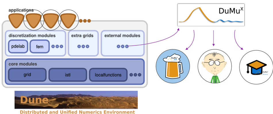
The DUNE Framework

• Developed by scientists at around 10 European research institutions.
• Separation of data structures and algorithms by abstract interfaces.
• Efficient implementation using generic programming techniques.
• Reuse of existing FE packages with a large body of functionality.
• Current stable release: 2.9 (November 2022).

DUNE Core Modules

• dune-common: basic classes
• dune-geometry: geometric entities
• dune-grid: abstract grid/mesh interface
• dune-istl: iterative solver template library
• dune-localfunctions: finite element shape functions

Overview

• DuMu^x: DUNE for Multi-{Phase, Component, Scale, Physics, \(\text{...}\)} flow and transport in porous media.
• Goal: sustainable, consistent, research-friendly framework for the implementation and application of FV discretization schemes, model concepts, and constitutive relations.
• Developed by more than 30 PhD students and post docs, mostly at LH² (Uni Stuttgart).

Applications

• gas (CO₂, H₂, CH₄, \(\text{...}\)) storage scenarios
• environmental remediation problems
• transport of substances in biological tissue
• subsurface-atmosphere coupling (Navier-Stokes / Darcy)
• flow and transport in fractured porous media
• root-soil interaction
• pore-network modelling
• developing new finite volume schemes

DuMu^x Modules

• dumux-lecture: example applications for lectures offered by LH², Uni Stuttgart
• dumux-pub/—: code and data accompanying a publication (reproduce and archive results)
• dumux-appl/—: Various application modules (many not publicly available, e.g. ongoing research)

Development History

• 01/2007: Development starts.
• 07/2009: Release 1.0.
• 09/2010: Split into stable and development part.
• 12/2010: Anonymous read access to the SVN trunk of the stable part.
• 02/2011: Release 2.0, \(\text{...}\), 10/2017: Release 2.12.
• 09/2015: Transition from Subversion to Git.
• 12/2018: Release 3.0, \(\text{...}\), 07/2024: Release 3.9.

Funding

Efforts mainly funded through ressources at the LH²: Department of Hydromechanics and Modelling of Hydrosystems at the University of Stuttgart and third-party funding aquired at the LH²

Funding

We acknowledge funding that supported the development of DuMu^x in past and present:

Downloads and Publications

• More than 1000 unique release downloads.
• More than 250 peer-reviewed publications and PhD theses using DuMu^x.

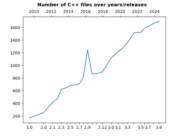
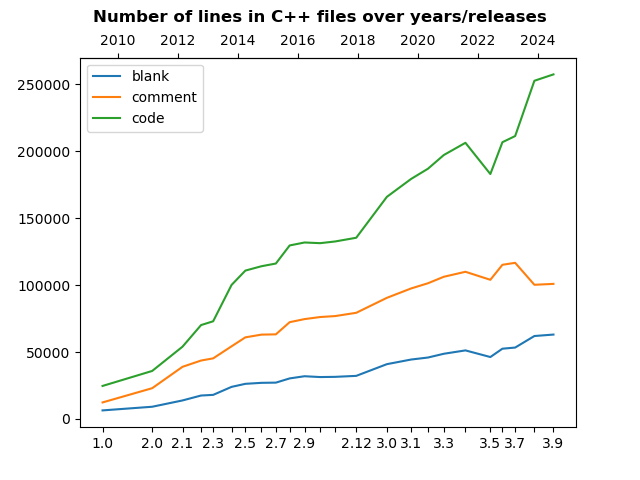
Evolution of C++ Files

Evolution of Code Lines

Mailing Lists and GitLab

• Mailing lists of DUNE (dune@dune-project.org) and DuMu^x (dumux@listserv.uni-stuttgart.de)
• GitLab Issue Tracker (https://git.iws.uni-stuttgart.de/dumux-repositories/dumux/issues)
• Get GitLab accounts (non-anonymous) for better access
  • DUNE GitLab (https://gitlab.dune-project.org/core)
  • DuMu^x GitLab (https://git.iws.uni-stuttgart.de/dumux-repositories/dumux)

Documentation

• Code documentation
  • DuMu^x (https://dumux.org/docs/doxygen/master/)
  • DUNE (https://dune-project.org/doxygen/)
• DuMu^x Examples (https://git.iws.uni-stuttgart.de/dumux-repositories/dumux/-/tree/master/examples#examples)
• DuMu^x Website (https://dumux.org/)

Mathematical Models

Preimplemented models:

• Flow in porous media (Darcy): Single and multi-phase models for flow and transport in porous materials.
• Free flow (Navier-Stokes): Single-phase models based on the Navier-Stokes equations.
• Shallow water flow: Two-dimensional shallow water flow (depth-averaged).
• Geomechanics: Models taking into account solid deformation of porous materials.
• Pore network: Single and multi-phase models for flow and transport in pore networks.

Flow in Porous Media

Darcy’s law

• Describes the advective flux in porous media on the macro-scale

• Single-phase flow \[ \mathbf{v} = - \frac{\mathbf{K}}{\mu} \left(\textbf{grad}\, p - \varrho \mathbf{g} \right) \]

• Multi-phase flow (phase \(\alpha\)) \[ \mathbf{v}_\alpha = - \frac{k_{r\alpha}}{\mu_\alpha} \mathbf{K} \left(\textbf{grad}\, p_\alpha - \varrho_\alpha \mathbf{g} \right) \] where \(k_{r\alpha}(S_\alpha)\) is the relative permeability, a function of saturation \(S_\alpha\).

• For non-creeping flow, Forchheimer’s law is available as an alternative.

1p – Single-Phase

• Uses standard Darcy approach for the conservation of momentum by default

• Mass continuity equation \[ \frac{\partial\left( \phi \varrho \right)}{\partial t} + \text{div} \left( \varrho \mathbf{v} \right) = q \]

• Primary variable: \(p\)

• Further details can be found in the corresponding documentation

1pnc – Single-Phase, Multi-Component

• Uses standard Darcy approach for the conservation of momentum by default

• Transport of component \(\kappa \in \{\text{H2O}, \text{Air}, ...\}\) \[ \frac{\partial\left( \phi \varrho X^\kappa \right)}{\partial t} + \text{div} \left( \varrho X^\kappa \mathbf{v} - \varrho D^\kappa_\text{pm} \textbf{grad} X^\kappa \right) = q \]

• Closure relation: \(\sum_\kappa X^\kappa = 1\)

• Primary variables: \(p\) and \(X^\kappa\)

• Further details can be found in the corresponding documentation

1pncmin – with Fluid-Solid Phase Change

• Transport equation for each component \(\kappa \in \{\text{H2O}, \text{Air}, ...\}\) \[ \frac{\partial \left( \varrho_f X^\kappa \phi \right)}{\partial t} + \text{div} \left( \varrho_f X^\kappa \mathbf{v} - \mathbf{D_\text{pm}^\kappa} \varrho_f \textbf{grad}\, X^\kappa \right) = q_\kappa \]

• Mass balance solid phases \[ \frac{\partial \left(\varrho_\lambda \phi_\lambda \right)}{\partial t} = q_\lambda \]

• Primary variables: \(p\), \(X^k\) and \(\phi_\lambda\)

• Further details can be found in the corresponding documentation

2p – Two-Phase Immiscible

• Uses standard multi-phase Darcy approach for the conservation of momentum by default

• Conservation of the phase mass of phase \(\alpha \in \{\text{w}, \text{n}\}\) \[ \frac{\partial \left(\phi \varrho_\alpha S_\alpha \right)}{\partial t} + \text{div} \left(\varrho_\alpha \mathbf{v}_\alpha \right) = q_\alpha \]

• Constitutive relations: \(p_\text{c} := p_\text{n} - p_\text{w} = p_\text{c}(S_\text{w})\), \(k_{r\alpha}\) = \(k_{r\alpha}(S_\text{w})\)

• Physical constraint (void space filled with fluid phases): \(S_\text{w} + S_\text{n} = 1\)

• Primary variables: \(p_\text{w}\), \(S_\text{n}\) or \(p_\text{n}\), \(S_\text{w}\)

• Further details can be found in the corresponding documentation

2pnc – Two-Phase Compositional

• Transport equation for each component \(\kappa \in \{\text{H2O}, \text{Air}, ...\}\) in phase \(\alpha \in \{\text{w}, \text{n}\}\) \[ \begin{aligned} \frac{\partial \left( \sum_\alpha \varrho_\alpha X_\alpha^\kappa \phi S_\alpha \right)}{\partial t} &+ \sum_\alpha \text{div}\left( \varrho_\alpha X_\alpha^\kappa \mathbf{v}_\alpha - \mathbf{D_{\alpha, pm}^\kappa} \varrho_\alpha \textbf{grad}\, X^\kappa_\alpha \right) = \sum_\alpha q_\alpha^\kappa \end{aligned} \]

• Constitutive relation: \(p_\text{c} := p_\text{n} - p_\text{w} = p_\text{c}(S_\text{w})\), \(k_{r\alpha}\) = \(k_{r\alpha}(S_\text{w})\)

• Physical constraints: \(S_\text{w} + S_\text{n} = 1\) and \(\sum_\kappa X_\alpha^\kappa = 1\)

• Primary variables: depending on the phase state

• Further details can be found in the corresponding documentation

2pncmin

• Transport equation for each component \(\kappa \in \{\text{H2O}, \text{Air}, ...\}\) \[ \begin{aligned} \frac{\partial \left( \sum_\alpha \varrho_\alpha X_\alpha^\kappa \phi S_\alpha \right)}{\partial t} &+ \sum_\alpha \text{div}\left( \varrho_\alpha X_\alpha^\kappa \mathbf{v}_\alpha - \mathbf{D_{\alpha, pm}^\kappa} \varrho_\alpha \textbf{grad}\, X^\kappa_\alpha \right)= \sum_\alpha q_\alpha^\kappa \end{aligned} \]

• Mass balance solid phases \[ \frac{\partial \left(\varrho_\lambda \phi_\lambda \right)}{\partial t} = q_\lambda \quad \forall \lambda \in \Lambda \] for a set of solid phases \(\Lambda\) each with volume fraction \(\varrho_\lambda\)

• Source term models dissolution/precipiation/phase transition fluid ↔︎ solid

• Further details can be found in the corresponding documentation

3p – Three-Phase Immiscible

• Uses standard multi-phase Darcy approach for the conservation of momentum by default

• Conservation of the phase mass of phase \(\alpha \in \{\text{w}, \text{g}, \text{n}\}\) \[ \frac{\partial \left( \phi \varrho_\alpha S_\alpha \right)}{\partial t} - \text{div} \left( \varrho_\alpha \mathbf{v}_\alpha \right) = q_\alpha \]

• Physical constraint: \(S_\text{w} + S_\text{n} + S_g = 1\)

• Primary variables: \(p_\text{g}\), \(S_\text{w}\), \(S_\text{n}\)

• Further details can be found in the corresponding documentation

3p3c – Three-Phase Compositional

• Transport equation for each component \(\kappa \in \{\text{H2O}, \text{Air}, \text{NAPL}\}\) in phase \(\alpha \in \{\text{w}, \text{g}, \text{n}\}\) \[ \begin{aligned} \frac{\partial \left( \phi \sum_\alpha \varrho_{\alpha,\text{mol}} x_\alpha^\kappa S_\alpha \right)}{\partial t}&+ \sum_\alpha \text{div} \left( \varrho_{\alpha,\text{mol}} x_\alpha^\kappa \mathbf{v}_\alpha - D_\text{pm}^\kappa \frac{1}{M_\kappa} \varrho_\alpha \textbf{grad} X^\kappa_{\alpha} \right) = q^\kappa \end{aligned} \]

• Physical constraints: \(\sum_\alpha S_\alpha = 1\) and \(\sum_\kappa x^\kappa_\alpha = 1\)

• Primary variables: depend on the locally present fluid phases

• Further details can be found in the corresponding documentation

Other Porous-Medium Flow Models

• For other porous-medium flow models, we refer to the Doxygen documentation:

  • 2p1c
  • 2p2c
  • 3pwateroil
  • co2
  • mpnc
  • nonequilibrium
  • richards
  • richardsnc
  • tracer

Non-Isothermal (Equilibrium)

• Local thermal equilibrium assumption

• One energy conservation equation for the porous solid matrix and the fluids

  \[ \begin{aligned}\frac{\partial \left( \phi \sum_\alpha \varrho_\alpha u_\alpha S_\alpha \right)}{\partial t} &+ \frac{\partial \left(\left(1 - \phi \right)\varrho_s c_s T \right)}{\partial t} + \sum_\alpha \text{div} \left( \varrho_\alpha h_\alpha \mathbf{v}_\alpha \right) - \text{div} \left(\lambda_\text{pm} \textbf{grad}\, T \right) = q^h \end{aligned} \]

• Specific internal energy \(u_\alpha = h_\alpha - p_\alpha / \varrho_\alpha\)

• Can be added to other models, additional primary variable temperature \(T\)

• Further details can be found in the corresponding documentation

Free Flow (Navier-Stokes)

• Stokes equation
• Navier-Stokes equations
• Energy and component transport

Reynolds-Averaged Navier-Stokes (RANS)

• Momentum balance equation for a single-phase, isothermal RANS model

  \[ \frac{\partial \left(\varrho \textbf{v} \right)}{\partial t} + \nabla \cdot \left(\varrho \textbf{v} \textbf{v}^{\text{T}} \right) = \nabla \cdot \left(\mu_\textrm{eff} \left(\nabla \textbf{v} + \nabla \textbf{v}^{\text{T}} \right) \right) - \nabla p + \varrho \textbf{g} - \textbf{f} \]

• The effective viscosity is composed of the fluid and the eddy viscosity

  \[ \mu_\textrm{eff} = \mu + \mu_\textrm{t} \]

• Various turbulence models are implemented

• More details can be found in the Doxygen documentation

Other Models

• For other models, we refer to the Doxygen documentation:

  • Shallow water
  • Geomechanics
  • Pore network

Your Model Equations?

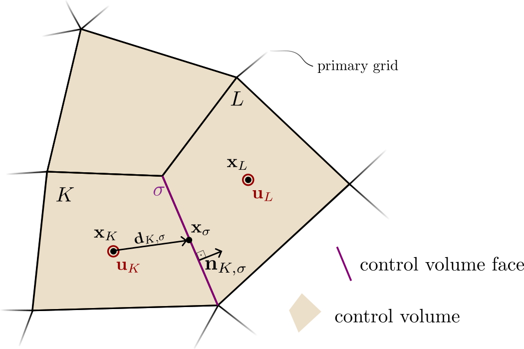
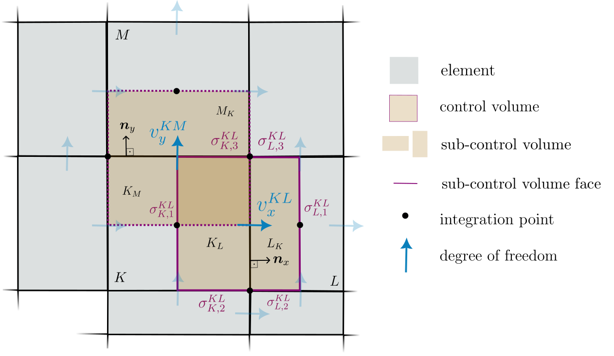
Cell-centered Finite Volume Methods

• Elements of the grid are used as control volumes
• Discrete values represent control volume average
• Two-point flux approximation (TPFA)
  • Simple and robust but not always consistent
• Multi-point flux approximation (MPFA)
  • A consistent discrete gradient is constructed

Two-Point Flux Approximation (TPFA)

Multi-Point Flux Approximation (MPFA)

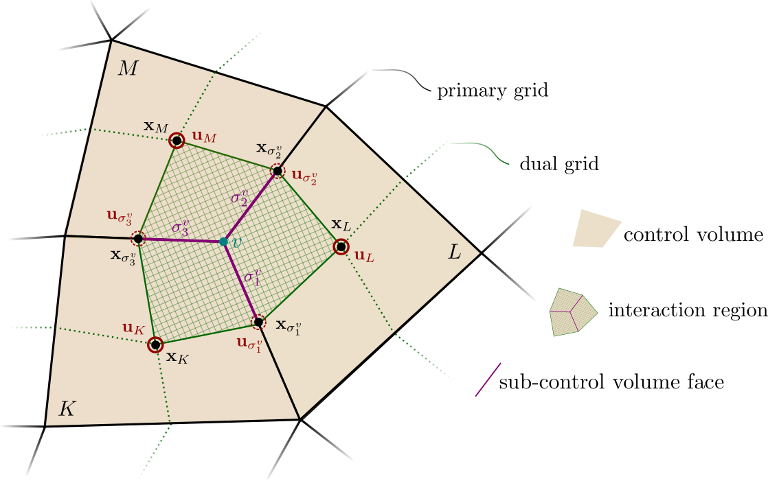
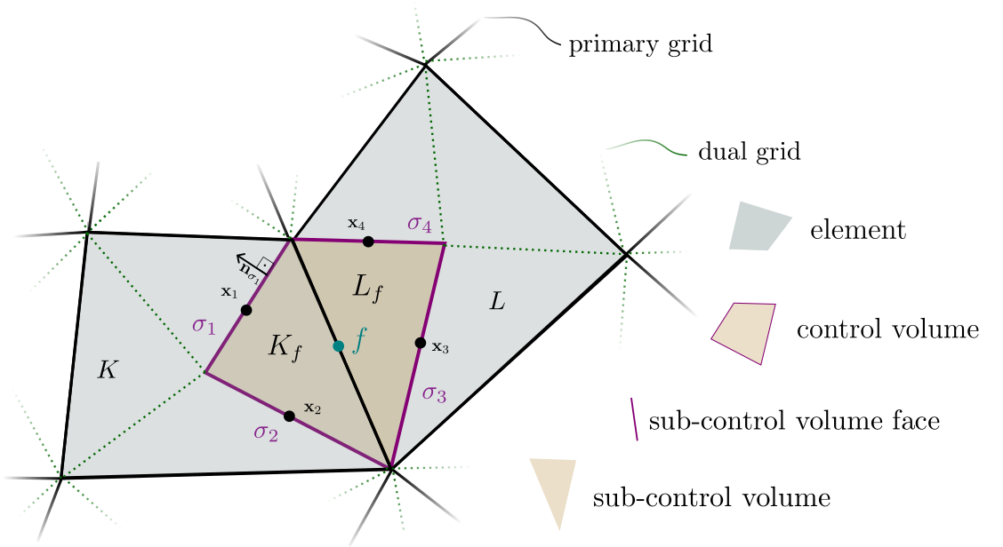
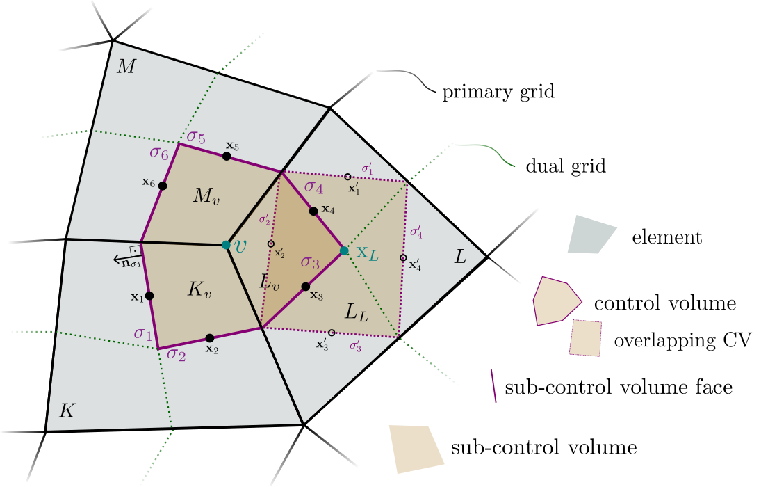
Control-Volume Finite Element Methods

• Model domain is discretized using a FE mesh
• Secondary FV mesh is constructed → control volume/box
• Control volumes (CV) split into sub control volumes (SCVs)
• Faces of CV split into sub control volume faces (SCVFs)
• Unites advantages of finite-volume (simplicity) and finite-element methods (flexibility)
  • Unstructured grids (from FE method)
  • Mass conservation (from FV method)

Box Method

Vertex-centered finite volumes / control volume finite element method with piecewise linear polynomial functions (\(\mathrm{P}_1/\mathrm{Q}_1\))

Diamond Scheme

Face-centered finite-volume scheme based on non-conforming finite-element spaces

PQ1 Bubble Scheme

Control-volume finite element scheme based on \(\mathrm{P}_1/\mathrm{Q}_1\) basis functions with enrichment by a bubble function

Finite Volume Method on Staggered Control Volumes

• Uses a finite volume method with different staggered control volumes for different equations
• Fluxes are evaluated with a two-point flux approximation
• Robust and mass conservative
• Restricted to structured grids (tensor-product structure)

Staggered Grid Discretization

Model Components

• Typically, the following components have to be specified
  • Model: Equations and constitutive models
  • Assembler: Key properties (Discretization, Variables, LocalResidual)
  • Solver: Type of solution stategy (e.g. Newton)
  • LinearSolver: Method for solving linear equation systems (e.g. direct / Krylov subspace methods)
  • Problem: Initial and boundary conditions, source terms
  • TimeLoop: For time-dependent problems
  • VtkOutputModule / IOFields: For VTK output of the simulation

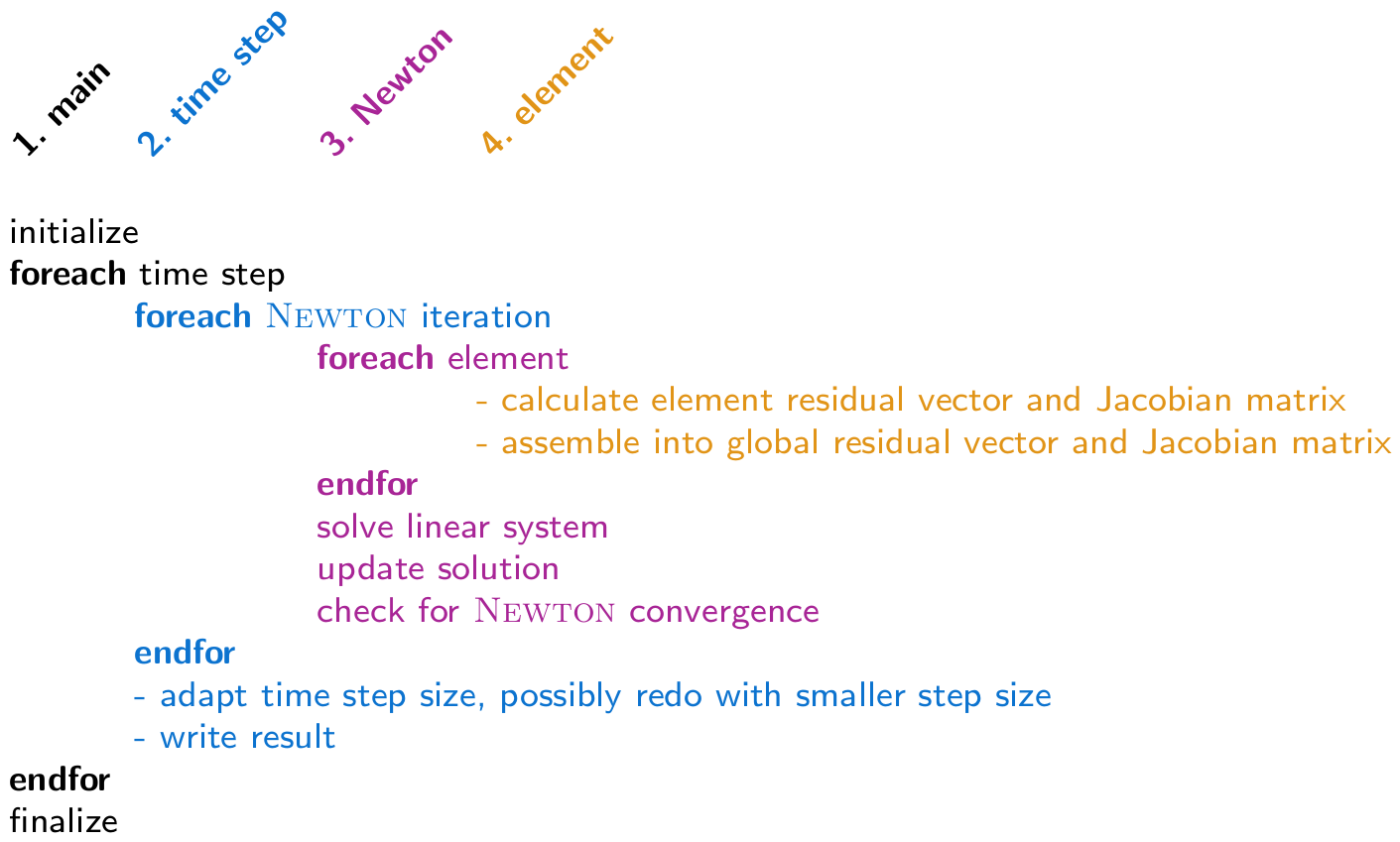
Simulation Flow