Active learning: iteratively expanding the training set

Active learning (AL), also called sequential training, is the iterative choice of additional training samples after the initial training of a surrogate model. The new samples can be chosen in an explorative manner or by exploiting available data and properties of the surrogate. The relevant functions are contained in the class bayesvalidrox.surrogate_models.sequential_design.SequentialDesign and bayesvalidrox.surrogate_models.exploration.Exploration.

Warning

Exploration with ‘voronoi’ is disabled for release v1.1.0!

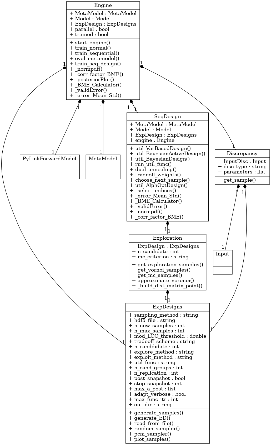
In BayesValidRox AL is realized by additional properties of the bayesvalidrox.surrogate_models.exp_designs.ExpDesigns and bayesvalidrox.surrogate_models.engine.Engine classes without any changes to the surrogate model.

Exploration, exploitation and tradeoff

Exploration methods choose the new samples in a space-filling manner, while exploitation methods make use of available data or properties of the surrogate models, such as the estimated surrogate standard deviation. Exploration methods in BayesValidRox include random or latin-hypercube sampling, voronoi sampling, choice based on leave-one-out cross validation or dual-annealing. Exploitation can be set to Bayesian designs, such as Bayesian3 Active Learning, or variance-based designs.

The tradeoff between exploration and exploitation is defined by tradeoff-schemes, such as an equal split, epsilon-decreaseing or adaptive schemes.

Example

We take the engine from Training surrogate models and change the settings to perform sequential training.

This mainly changes the experimental design. For this example we start with the 10 initial samples from Training surrogate models and increase them iteratively to the number of samples given in n_max_samples. The parameter n_new_samples sets the number of new samples that are chosen in each iteration, while mod_LOO_threshold sets an additional stopping condition.

>>> ExpDesign.n_max_samples = 14
>>> ExpDesign.n_new_samples = 1
>>> ExpDesign.mod_LOO_threshold = 1e-16

Here we do not set a tradeoff_scheme. This will result in all samples being chosen based on the exploration weights.

>>> ExpDesign.tradeoff_scheme = None

As the proposed samples come from the exploration method, we still need to define this.

>>> ExpDesign.explore_method = 'random'
>>> ExpDesign.n_canddidate = 1000
>>> ExpDesign.n_cand_groups = 4

For the exploitation method we use a variance-based method, as no data is given.

>>> ExpDesign.exploit_method = 'VarOptDesign'
>>> ExpDesign.util_func = 'EIGF'

Once all properties are set, we can assemble the engine and start it. This time we use train_sequential.

>>> Engine_ = Engine(MetaMod, Model, ExpDesign)
>>> Engine_.train_sequential()