Training surrogate models
Surrogate models, also called metamodels, are models that are built on evaluations of full models with the goal to capture the full model behaviour, but reduce the cost of evaluations. The surrogate models are trained on datasets \(\mathcal{D}=(x_i, y_i)_{i=1,\dots,M}\) that consist of \(M\) samples of the uncertain parameters and the corresponding model outputs. We call this dataset the training data, with training samples \((x_i)_{i=1,\dots,M}\).
MetaModel options
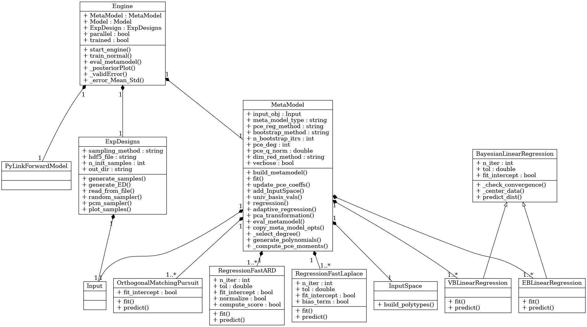
BayesValidRox creates surrogate models as objects of classes that inherit from the class bayesvalidrox.surrogate_models.meta_model.MetaModel.
Training is performed by the class bayesvalidrox.surrogate_models.engine.Engine.
The general metamodel interface and functionalities that BayesValidRox expects are contained in the template class bayesvalidrox.surrogate_models.meta_model.MetaModel.
This class also includes general functionalities for dimensionality reduction, bootstrapping and the calculation of the moments of the metamodel outputs.
Dimensionality reduction on outputs can be performed with Principal Component Analysis (PCA).
In this case, PCA is applied on the set of surrogates built for the x_values defined in the model.
If bootstrapping is used, multiple surrogates will be created based on bootstrapped training data, and jointly evaluated. The final outputs will then be the mean and standard deviation of their approximations.
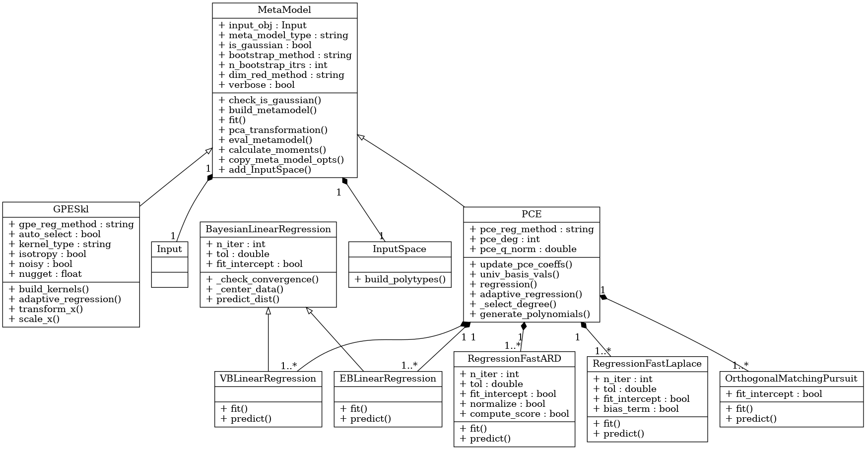
In BayesValidRox two main types of surrogate model are available, Polynomial Chaos Expansion (PCE) and Gaussian Processes Emulators (GPE). The Polynomial Chaos Expansion (PCE) and its variant the arbitrary Polynomial Chaos Expansion (aPC) build polynomials from the given distributions of uncertain inputs. Gaussian processes Emulators (GPE) give kernel-based representations of the model results.
Polynomial Chaos Expansion
The class bayesvalidrox.surrogate_models.polynomial_chaos.PCE is a polynomial-based metamodel.
We provide a broad range of regression methods for useage with PCE-surrogates that can be set by the parameter PCE.pce_reg_method, including
Ordinary Least Squares (
ols)Pseuso-inverse (
pinv)Bayesian Ridge Regression (
brr)Bayesian ARD Regression (
ard)Fast Bayesian ARD Regression (
fastard)Fast Laplace Regression (
bcs)Least angle regression (
lars)Lasso-Least angle regression (
lassolars)Lasso-Least angle regression with cross validation (
lassolarscv)Variational Bayesian Learning (
vbl)Emperical Bayesian Learning (
ebl)Orthogonal Matching Pursuit (
omp)Stochastic Gradient Descent (
sgdr)
The surrogate outputs a mean approximation and, depending on the chosen regression method, the associated standard deviation.
For aPCE-type surrogate models, their derivatives can be evaluated with the function PCE.derivative().
Gaussian Process Emulator
Our current GPE implementation with the class bayesvalidrox.surrogate_models.gaussian_process_sklearn.GPESkl is based on the scikit-learn Gaussian Process Regressor. —https://scikit-learn.org/stable/modules/generated/sklearn.gaussian_process.GaussianProcessRegressor.html
It allows for the following kernel types:
Radial Basis Function (
rbf)Matérn (
matern)Rational Quadratic (
rq)
If the training data is assumed to be noisy, then _kernel_noise can be set, which will add a White Noise kernel.
Mixture forms
The metamodel classes can be combined to form new metamodel types.
In BayesValidRox a combination class bayesvalidrox.surrogate_models.pce_gpr.PCEGPR exists, which uses PCE for a global approximation and builds a GP on its residual error.
Training with the engine
For training a surrogate model we use an object of class bayesvalidrox.surrogate_models.engine.Engine.
This needs to be given three things: the metamodel itself, the model that the metamodel should replace, and the experimental design that matches the uncertain inputs for the model and metamodel.
The standard method of training the surrogate is performed by the function train_normal().
Other available training methods in BayesValidRox are presented in Active learning: iteratively expanding the training set.
For training the engine performs three main steps.
Generating training samples from the experimental design.
Evaluating the model on the training samples.
Fitting the surrogate to the training dataset.

Example
We now build a polynomial chaos surrogate model for the simple model from Models using the experimental design from Priors, input space and experimental design.
For this we need the classes bayesvalidrox.surrogate_models.meta_model.MetaModel and bayesvalidrox.surrogate_models.engine.Engine.
>> from bayesvalidrox import PCE, Engine
First we set up the surrogate model and set the uncertain parameters defined in Inputs as its input parameters.
>>> meta_model = PCE(inputs)
Then we specify what type of surrogate we want and its properties. Here we use an aPCE with maximal polynomial degree 3 and use FastARD as the regression method. We set the value of the q-norm truncation scheme to 0.9. This combination will give us a sparse aPCE.
>>> meta_model.meta_model_type = 'aPCE'
>>> meta_model.pce_reg_method = 'FastARD'
>>> meta_model.pce_deg = 3
>>> meta_model.pce_q_norm = 0.85
Before we start the actual training we set n_init_samples to our wanted number of training samples.
>>> exp_design.n_init_samples = 10
With this the experimental design will generate 10 samples according to our previously set sampling method.
Alternatively we can set the training samples by hand using ExpDesigns.x.
If we also want to assign the training outputs explicitly, we do this via setting ExpDesigns.y.
>>> exp_design.x = samples
Now we create an engine object with the model, experimental design and surrogate model, and run the training.
>>> engine = Engine(meta_model, model, exp_design)
>>> engine.train_normal()
We can evaluate the trained surrogate model via the engine, or directly. The evaluations return the mean approximation of the surrogate and its associated standard deviation. Evaluation via the surrogate model can make use of the sampling in the experimental design,
>>> mean, stdev = engine.eval_metamodel(nsamples = 10)
while for direct evaluation the exact set of samples has to be given.
>>> mean, stdev = engine.meta_model.eval_metamodel(samples)