Postprocessing

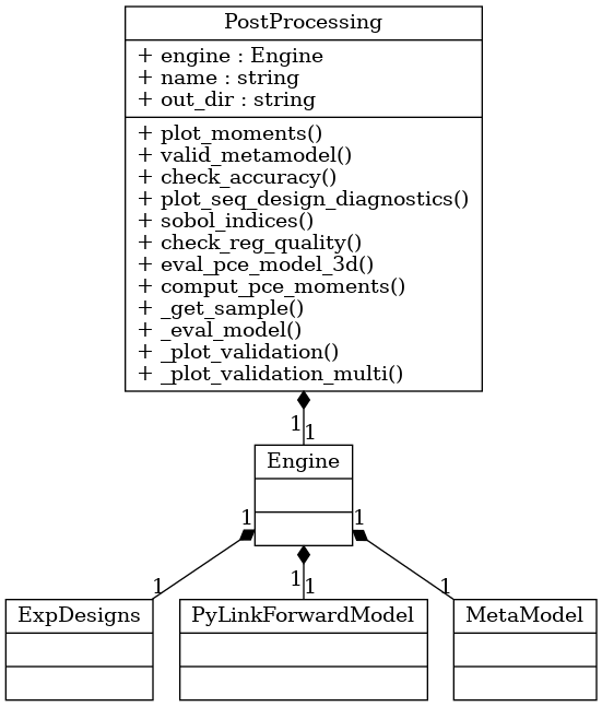
Postprocessing refers to evaluations and checks performed on a model to get an understanding of its properties and estimate its quality. The BayesValidRox class bayesvalidrox.post_processing.post_processing.PostProcessing includes functions for evaluating and visualizing surrogate models.

• plot_expdesign: Visualizing the set marginals and training points

• plot_moments: Visualizing the moments of the outputs of a surrogate model

• validate_metamodel: Computing validation scores and visualizing the scores and the surrogate outputs; this function also calls plot_correl, plot_seq_design_diagnostics, plot_validation_outputs and plot_residual_hist

Global sensitivity analysis can be performed by calculating the Sobol’ indices or the AMA indices via their respective classes, bayesvalidrox.post_processing.sobol.Sobol and bayesvalidrox.post_processing.ama.AMA. Both classes inherit their structure from the class bayesvalidrox.post_processing.gsa.GSA, which additionally contains general functions for storage and visualization of the indices.

The generalized calculation of the indices is based on MC-samples generated from the engine input space, which are binned to calculate the conditional moments. As this binning is feasible only along individual input dimensions, the MC-based calculation of the indices returns only first-order effects. For the Sobol’ indices, an additional calculation directly from the PCE coefficients is available, which additionally returns higher-order effects.

Example

We want to compare out trained surrogate from Active learning: iteratively expanding the training set against its original model using the class bayesvalidrox.post_processing.post_processing.PostProcessing.

>>> from bayesvalidrox import PostProcessing

The postprocessing object expects the full engine. This allows it to perform both sampling, running the model and running the surrogate model.

>>> post = PostProcessing(engine, out_format='png')

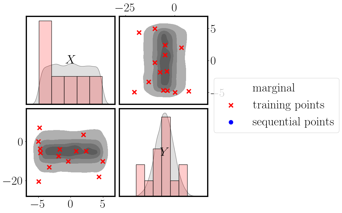
We start by visualizing the set marginals and the training points.

>>> post.plot_expdesign(show_samples = True)

If not specified otherwise, the plots are stored in the folder Outputs_PostProcessing_model.

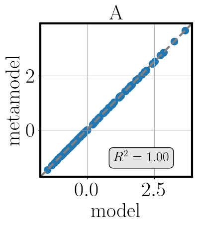
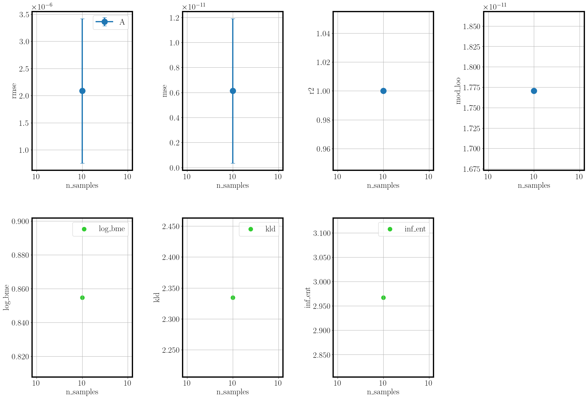
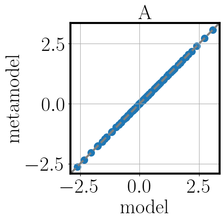
To gain an understanding of the approximation quality we use the function validate_metamodel. Tihs function generates validation samples, then applies the applicable validation metrics and visualizes the results. The validation metrics are selected based on the available data and include the RMSE, MSE and R2 values, mean and standard deviation errors of the moments against references, and Bayesian metrics such as BME, DKL and information entropy, if a reference observation is given.

>>> post.validate_metamodel(n_samples=10)

The visual comparison of model and metamodel results is saved in the folder Outputs_PostProcessing_model.

To calculate the Sobol’ and AMA indices we need the classes bayesvalidrox.post_processing.sobol.Sobol and bayesvalidrox.post_processing.ama.AMA.

>>> from bayesvalidrox import Sobol, AMA

For the Sobol’ indices we give the engine with a PCE-type surrogate model. The indices are calculated, stored and visualized by calling the function calc_indices.

>>> sob = Sobol(engine, out_format="png")
>>> indices = sob.calc_indices()

The AMA indices can be calculated using the same syntax. As these are MC-based for all surrogate types, we additionally set the number of MC-samples here.

>>> ama = AMA(engine, n_mc = 100000)
>>> indices = ama.calc_indices()

If not specified otherwise, the indices and plots are stored in subfolders Outputs_PostProcessing_model\sobol and Outputs_PostProcessing_model\ama.