Bayesian inference

With Bayesian inference we ask the question ‘how does our understanding of the inputs change given some observation of the outputs of the model?’, i.e. we perform an updating step of the prior distributions to posterior, based on some observations. Bayesvalidrox provides a dedicated class to perform this task, bayesvalidrox.bayes_inference.bayes_inference.BayesInference, which uses bayesvalidrox.bayes_inference.post_sampler.PostSampler objects to generate posterior samples.

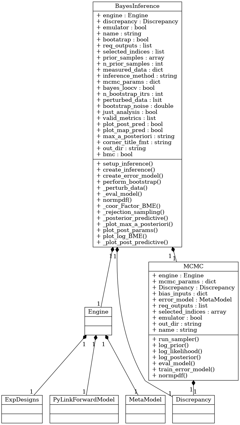
In addition to inference, the class bayesvalidrox.bayes_inference.bayes_inference.BayesInference can also be used to validate a model or surrogate model on given observations by estimating the BME. Both options use an observation, to be given as an object of the class bayesvalidrox.bayes_inference.observation.Observation. For the analysis, the observation can be perturbed using added Gaussian noise, or bootstrapped with leave-one-out cross-validation.

Sampler classes

Bayesvalidrox supports two options for generating posterior samples, rejection-sampling and MCMC. Both of them are given in separate child classes of the bayesvalidrox.bayes_inference.post_sampler.PostSampler class.

Additional parameters for MCMC can be given to bayesvalidrox.bayes_inference.bayes_inference.BayesInference as a dictionary called mcmc_params and can include

• prior_samples: initial samples

• nsteps: number of steps

• nwalkers: number of walkers

• nburn: length of the burn-in

• moves: function to use for the moves, e.g. taken from emcee

• mp: setting for multiprocessing

• verbose: verbosity

Example

For this example we add the following imports.

>>> from bayesvalidrox import Observation, BayesInference

In order to run Bayesian inference we first need to provide an observation. For this example we take an evaluation of the model on some chosen sample and create an Observation object. As this expects a 1D-array for each output key, we need to change the format slightly. We also add an estimation of the measurement uncertainty as a standard deviation in observation.sigma2, here we set it to 0.01 of the measurement values.

>>> true_sample = np.array([[2, 2]])
>>> obs_data = model.run_model_parallel(true_sample)[0]
>>> sigma2 = {}
>>> for key in obs_data:
>>>     if key != 'x_values':
>>>             obs_data[key] = obs_data[key][0]
>>>             sigma2[key] = obs_data[key]*0.01
>>> observation = Observation(data = obs_data, sigma2=sigma2)

Now we can initialize an object of class bayesvalidrox.bayes_inference.bayes_inference.BayesInference with all the wanted properties. This object has to be given our Engine. If it should use the surrogate during inference, set use_emulator to True, otherwise the model will be evaluated directly. We also set the defined observation. and set post if posterior predictions should be visualized.

>>> bayes = BayesInference(Engine_, observation)
>>> bayes.use_emulator = True
>>> bayes.plot = True

In order to run with rejection sampling, we set the inference_method.

>>> bayes.inference_method = 'rejection'

If the sampling should be done with MCMC, then the inference_method is set to 'MCMC' and additional properties are given in mcmc_params. For this example we use the python package emcee to define the MCMC moves.

>>> bayes.inference_method = 'MCMC'
>>> import emcee
>>> bayes.mcmc_params = {
>>>     'nsteps': 1e4,
>>>     'nwalkers': 30,
>>>     'moves': emcee.moves.KDEMove(),
>>>     'mp': False,
>>>     'verbose': False
>>>     }

Then we run the inference.

>>> bayes.run_inference()

If the output directory bayes.out_dir is not set otherwise, the outputs are written into the folder Outputs_Bayes_model_Calib. This folder includes the posterior distribution of the input parameters, as well as the predictions resulting from the mean of the posterior. For inference with MCMC, chain diagnostics are also written out in the console.

---------------Posterior diagnostics---------------
Mean auto-correlation time: 2.057
Thin: 1
Burn-in: 4
Flat chain shape: (13380, 1)
Mean acceptance fraction*: 0.752
Gelman-Rubin Test**:  [1.001]

* This value must lay between 0.234 and 0.5.
** These values must be smaller than 1.1.
--------------------------------------------------

For validation, we perturb the observations with Gaussian noise, generating 500 noisy versions.

>>> bayes.bootstrap_method = 'gaussian'
>>> bayes.n_bootstrap_itrs = 500
>>> bayes.bootstrap_noise = 0.2

We can calculate additional metrics for validation, by adding them to the valid_metrics list. Options include the Kullback-Leibler Divergence ('KLD') and Information entropy ('inf_entropy').

>>> bayes.valid_metrics = ['kld', 'inf_entropy']

Now we run the validation, which will return the log-BME of the model (or surrogate model) on the observations.

>>> log_bme = bayes.run_validation()

If the output directory bayes.out_dir is not set otherwise, the outputs are written into the folder Outputs_Bayes_model_Valid, and the log-BME is visualized. The additional metrics are stored in bayes.kld and bayes.inf_entropy.